This page illustrates with some examples the different results you can achieve
using the algorythm present on the page
HDR on line,
depending on the number of the starting images and the gradient shape chosen.
It is possible to choose between three local methods, i.e. which calculate the pixels
of the final image one pixel at a time (taking into consideration at best the ones
immediately adiacent like in the case of the third one):
- Linear gradient
- Spherical gradient (ok, in reality it just has the shape of a quarter of a circle,
but spherical sounds very good!)
- Adaptive gradient
The following pictures illustrate the two gradient types and the meaning of the parameters
you can work on. The first image refer to the case of two pictures, the other two to the
case of three pictures.
Furthermore there is also (in the case of three starting pictures) a nonlocal method,
which calculates the pixels of the final image based on the information contained
in the starting pictures as a whole:
LOCAL METHODS
In the first case the percentage of information coming from the High Light picture
increases linearly with the decreasing of the pixel brightness. In the second case,
instead, the information of the Low Light picture is used almost only in the darker
parts of the image. In the third case the system chooses pixel per pixel the more suitable
gradient of the two above. For each pixel the system calculates the luminosity
of the square of 25 pixels in the center of which the pixel is located and then
the standard deviation of the luminosity in these 25 pixels, both in the case of
linear gradient and of spherical gradient. Finally it assigns a weight to each of the two
gradient types, proportionally to found stansard deviations. The goal is to better preserve
the microcontrast.
This calculations has two limitations:
- Together with the microcontrast also the noise is preserved
- The system is able to compare only the two extremes: all pixel determined according
linear gradient or all pixels determined according spherical gradient.
The real final result, which stays between them, is not considered.
The three starting pictures in the table below were taken on a scale of 2 stops
(-1 stop / 0 / +1 stop).
We raccomand to open the pictures at full size to better appreciate the differences!
NON LOCAL METHOD (MIXED INTERPOLATIVE)
This method arises from the need to preserve the Luminosity gradient in some images with areas with little contrast and brightness such that the simple calculation pixel by pixel leads to flatten, when not even to invert, the brightness ratio between adjacent areas of the image. A problem
particularly frequent in the case of linear gradient.
The idea is to use the information contained in the other images to imagine the luminosity that
the pixels in the starting image should have, if the luminosity was not limited to the 0-442 range.
(Remember that the luminosity is the module of the vector that describes the pixel in the
three-dimensional RGB space).
It would be more intuitive to do this starting from the overexposed image, creating virtual pixels with
luminosity > 442 in the image areas where the luminosity has reache saturation.
Once these virtual pixels have been calculated, the brightness of all the pixels would be scaled
proportionally to each other, so as to bring them all in the 0-442 range.
Unfortunately, it has been verified that this leads to the emergence of terrible artifacts which make
the final image totally unusable.
Fortunately, the inverse way has proved to be practicable, that is starting from the underexposed image,
calculating virtual pixels with luminosity < 0 for areas where luminosity is below a certain luminosity
threshold ("Reference luminosity") and then scale all the luminosities upward, so as to bring the luminosity of the
darker pixels to zero.
This is made possible by the fact that on a double logarithmic scale the ratio between the luminosity of
the pixels of an image and the corresponding ones of the same framing exposed differently tend to be constant over almost everything
the luminosity range of the starting image. It however diverges at the two extremes, in the bright part because the luminosity
maximum converges for all the images to 442 (apart from the very dark ones that have no saturated parts),
on the dark side because where there is little light, the noise proportional to the exposure time becomes predominant.
The method is called mixed, because once the luminosity (ie its module) of the RGB vector is calculated for a given pixel,
its components (ie its orientation) are calculated according to the linear gradient method.
This has two advantages:
- Getting a more saturated image in the darker areas, as the saturation is less in the darkest areas of a photo
and it does not increase proportionally when the luminosity is increased.
- Reducing the signal to noise ratio, by taking more information where there is more
By varying the available parameters (Reference brightness and the two Delta Logs) it is possible to vary
significantly final result (although not always in a predictable way). In general, the increase in the value of these parameters
leads to a brighter final images. However, it is better to use the Preview function, before calculating the
final full size image!
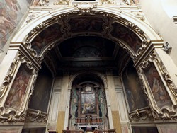
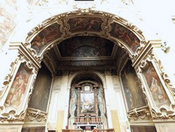
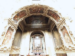
Below are some sample starting images with a particularly difficult picture (using local methods
many frescoes tend to disappear or otherwise to be distorted in their color relationships):
|
STARTING IMAGES
|
 |  |  |
|
|
Linear Gradient
|
Adaptiv Gradient
|
Mixed Interpolative Method
|
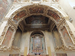 | 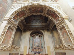 | 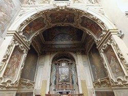 |
If you open the images obtained with the three different methods, you notice that the adaptive gradient provides more saturated colors,
but many of the frescoes have lost most of their details so to make the figures in them almost no longer recognizable.
On the contrary, the mixed interpolative method provides the maintenance of details, at the price, however, of
duller colors and darker parts in the shade. The result obtained, however, appears nevertheless more realistic, especially considering
that it can be later improved with any image processing program, for example Faststone.
(The spherical gradient has not been inserted, but the results it provides are similar to those of the linear gradient, but even worse.)
What is important to underline is that there is no method that is always the best. The most convenient choice
varies depending on the case and the only way is to try!